Basta!

Loudspeaker simulator

Technical documentation

Ó Tolvan Data 2005

2007-01-13

Basta!

Basta! is a computer program for simulation and measurement of loudspeaker systems. It can simulate closed, bass-reflex, 1-port bandpass and 2-port bandpass systems. It can derive amplitude and phase response as a function of frequency for these systems. It manages multiple elements, both in parallel and isobaric operation.

Simulation

The model used in Basta! assumes a signal (voltage) source followed by an optional set of active crossover filters, a power amplifier, a passive electric circuit which feeds a voltage to the loudspeaker. The loudspeaker feeds an acoustic flow into the box, which in turn feeds an acoustic flow into the radiation resistance. Some of this flow may originate directly from the loudspeaker. The power produced in the radiation resistance is the acoustic power generated by the system.

Block diagram for the Basta! simulation.

In the following, the parts of the simulation are described in detail.

Signal source

The signal source is a simple voltage source. By changing the voltage, the output level of the loudspeaker will change. The voltage can also be set to a negative value in order to simulate reversed polarity of the speaker.

Active filter

Active filters are typically connected before the power amplifier. Basta! allows high- and lowpass filters of order 1 to 4. A lookup table for butterworth (odd order) or linkwitz (even order) filters, is included.

The filters are realised as follows:

First order One first order link

Second order One second order link

Third order One second order link and one first order link

Fourth order Two second order links

First and second order links can typically be realised by means of operational amplifiers and a few passive components. In the following, examples are given on how to realise the circuitry.

First order low pass filter

The first order filter is realised by means of an RC link and a voltage follower.

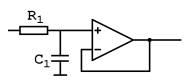
Example realisation of a first order low pass filter

The transfer function is

The cut-off frequency is given by

Select R₁=10 kW, and calculate C₁ = 1/(2pf₀R₁)

First order high pass filter

The first order filter is realised by means of an CR link and a voltage follower.

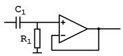
Example realisation of a first order high pass filter

The transfer function is

The cut-off frequency is given by

Select R₁=10 kW, and calculate C₁ = 1/(2pf₀R₁)

Second order low pass filter

The second order filter is realised by means of an RC network and a voltage follower.

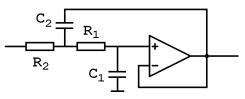
Example realisation of a second order low pass filter

The transfer function is

The cut-off frequency and Q value are given by

Select R₁ = R₂ = R =10 kW, calculate C₁ = Q/(pf₀R), C₂ = 1/(4pf₀RQ)

Second order high pass filter

The second order filter is realised by means of an RC network and a voltage follower.

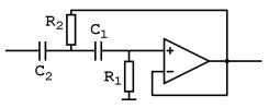
Example realisation of a second order high pass filter

The transfer function is

The cut-off frequency and Q value are given by

Select R₂ =10 kW, calculate R₁ = R₂/(4Q²) and

Third order filters

The third order filter is realised by cascading a first order filter with a second order filter.

Fourth order filters

The fourth order filter are realised by cascading two second order filters.

Power amplifier

For the normal configuration, the power amplifier has little purpose in Basta!. It is assumed to be an ideal voltage follower, ie gain =1 and output impedance = 0. However, when the AC-bass* configuration is simulated, an AC-bass network is connected to the output of the voltage follower.

It can be seen that if R_acneg equals -R_E of the voice coil, they will cancel, and L_ac and C_ac will have the same effect on the response as a spring and a mass on the mechanical side. R_ac will become the new effective voice coil resistance. Thus, the AC-bass principle can be used to control the apparent mechanical mass, compliance and lossiness, or in other words, f_s, V_as and Q_ts can be selected freely.

The AC-bass network is typically not built like the network above; it is normally included in the power amplifier using current feedback to design an output impedance like in the figure.

When the AC-bass network is used, all other filters are typically disabled. The only exception is the conjugate link, which can be utilised to reduce the effects of the voice coil inductance.

*AC-bass was first described in a master thesis by Karl-Erik Ståhl at the department of Speech, Music and Hearing, Royal Institute of Technology, Sweden. The principle was patented in the late 1970's and is user by Audio Pro AB under the name ACE-bassä. There are also products from Yamaha that use the principle. The patents have now expired, and as far as I understand anyone is free to use the concept.

Passive electric circuit

Between the driving amplifier and the loudspeaker, some passive electrical components can be added. This network consists of a set of optional parts; a freely configurable passive "advanced RLC network", a low-pass filter of order 0 to 4, a high-pass filter of order 0 to 4, an attenuation network and a conjugate link.

Circuit diagram of the passive network used in Basta! Some or all parts may be excluded.

Advanced RLC network

This network can be any combination of resistors, capacitors and/or inductors. The network has three pre-defined nodes, "in", "out", and "gnd", corresponding to its input, output and ground connections. Apart from these nodes, the network may contain additional internal nodes, which are identified by user-selected names.

In some cases, like the conjugate link, no separate in- and outputs are desired. If so, the input and outputs can be shorted. In this case "in" and "out" are treated as synonyms for the common node that is connected to the "hot" side of the network.

In principle, the remaining parts of the passive electric circuit can also be built as part of the advanced RLC network, but in many cases it is easier to use the pre-defined circuits, as follows.

Passive crossover filters

Passive low pass and high pass sections up to order 4 can be connected. The low pass section is formed by L_L1, C_L1, L_L2 and C_L2. Series resistances in the two coils are modelled through R_L1 and R_L2. The low pass filter is followed by a high pass filter consists of C_H1, L_H1, C_H2 and L_H2, and the series resistances of the coils are modelled through R_H1 and R_H2. For lower filter orders, some of the components are removed

Lowpass	0^th order	1^st order	2^nd order	3^rd order	4^th order
LL1	Short	USED	USED	USED	USED
RL1	Short	USED	USED	USED	USED
CL1	Open	Open	USED	USED	USED
LL2	Short	Short	Short	USED	USED
RL2	Short	Short	Short	USED	USED
CL2	Open	Open	Open	Open	USED

Highpass	0^th order	1^st order	2^nd order	3^rd order	4^th order
CH1	Short	USED	USED	USED	USED
LH1	Open	Open	USED	USED	USED
RH1	Open	Open	USED	USED	USED
CH2	Short	Short	Short	USED	USED
LH2	Open	Open	Open	Open	USED
RH2	Open	Open	Open	Open	USED

Design of the passive filters. For lower order filters, some of the components are shorted or left open.

A lookup table for Butterworth (odd order) or Linkwitz (even order) filters, is included The tables assume a resistive load, which means that the values of the components probably will need some manual tweaking to achieve the intended response of the loudspeaker system.

Attenuation network (L-pad)

The signal to the loudspeaker can be attenuated by the resistors Rs and Rp. The resistors are not used if theirs values are set to 0. These resistances together with R_L1 and R_L2 will affect the effective Q_ts value of the loudspeaker and can thus be utilised to fine tune the Q_ts value. It will, however also deteriorate the efficiency of the system since some power is lost in the resistances.

Conjugate link

To compensate for the voice coil inductance a conjugate link formed by R_EC and C_EC can be used. Their values can be calculated automatically from voice coil resistance and inductance, but given the lossy nature of the voice coil inductance, these values mostly need some manual tweaking to achieve an approximately flat and resistive impedance curve.

The purpose of the conjugate link is to provide the crossover filters with an approximately resistive load towards higher frequencies.

Loudspeaker

The loudspeaker is modelled using the electrical impedance of the voice coil via the resistance R_E and inductance L_E. This inductance can be modelled as lossy, see below. The electro-dynamic transducer is modelled by means of a gyrator with the gyration constant T=Bl. The mechanical system is modelled by the moving mass M_MS, the suspension compliance C_MS and mechanical damping R_MS. The mechanical velocity is then converted to an acoustic flow Q_s via the equivalent piston area S_s.

Equivalent circuit diagram of the loudspeaker element. To the left, variables and impedances are electrical, in the middle, they are mechanical, and to the left they are acoustic.

The following equations are used to determine the component values in the diagram:

where

f_s is the resonance of the loudspeaker element in free air

V_as is the equivalent volume of the cone suspension

T is the force factor AKA Bl

Q_ts is the total Q value of the loudspeaker element

R_E is the DC resistance of the voice coil

S_s is the equivalent piston area of the loudspeaker element

r_r is the piston radius corresponding to S_s

Note that the mechanical mass M_MS is reduced by the amount of the co-oscillating air for a piston in free air. Co-oscillating air is later added in terms of M_AL.

Voice coil losses

The voice coil inductance can be modelled as lossy. Measurement of real voice coils show that the impedance behaves far from a simple resistor in series with an inductance. A more appropriate model also takes into account "eddy currents" induced in the magnetic pole pieces in the loudspeaker. A much better model is to use this equation for the voice coil impedance

Where n is the loss factor. If n=1 the voice coil is lossless and the impedance is R_E+jwL_E, however most loudspeakers have a n value of 0.6 to 0.7. The main drawback with using this equation is that manufacturers rarely specify the voice coil inductance in this way. Thus in order to take advantage of the improved precision provided by the refined model, the simulation has to be matched against measured data, e.g. in terms of an impedance curve.

Voice coil temperature

The voice coil resistance R_e varies with temperature. Basta! can simulate this by assuming that the voice coil resistance is proportional to the absolute temperature. The Actual R_e is modelled as

where T is the temperature in °C. Modifying the temperature setting is equivalent to adding a series resistance, e.g. by the L-pad.

Box

The box can be either of a closed box, bass-reflex box, 1-ported band pass box or a 2-ported band pass box.

Closed box

The closed box is simulated by an acoustic compliance C_AV simulating the cavity and an acoustic resistance R_AV corresponding to resistive losses within the box, e.g. from damping material. Two masses M_AL corresponding to the co-oscillating air on the in- and outside of the box are included, as well as one radiation resistance R_AL. M_AL and R_AL are derived from the radiation impedance of a pulsating sphere. The power dissipated in the radiation resistance corresponds to the radiated acoustic power of the system. The component values are calculated as follows:

where

V_b is the box volume

Q_b is the Q-value that would occur if f_s was determined by C_AV and R_AV was the only loss

r_s is the equivalent radius of the pulsating half-sphere.

The closed box and the equivalent circuit diagram of its acoustic load.

The simplified transfer function of the closed box design behaves like a second order high pass filter with a slope of 12 dB/octave at low frequencies.

Bass-reflex box

The bass-reflex box is simulated using the same connection of the acoustic compliance C_AV and damping R_AV as for the closed box. Part of the flow into the box, passes out through the tube, and thus the vent is connected in parallel with C_AV and R_AV. The radiation resistance is connected in the box branch since the net flow into the surroundings is Q_s-Q_B, ie the difference between the flow out of the loudspeaker element and the flow out of the vent. This net flow forms the useful flow of the system, and thus the radiation resistance is connected there. In case of the more advanced vent model, the third connection of the vent ensures that Q_s-Q_B rather than Q_s-Q_A flows through the radiation resistance, see diagram. The radiation resistance is now calculated using the radius of the loudspeaker, since the loudspeaker delivers the major part of the flow at high frequencies. The part of the radiation resistance that contains the radiator radius is only important towards higher frequencies.

The bass-reflex box and the equivalent circuit diagram of its acoustic load.

The simplified transfer function of the bass-reflex design behaves like a fourth-order high pass filter with a slope of 24 dB/octave at low frequencies.

1-ported band pass box

The simulation of the 1-ported band pass box is similar to the bass-reflex box, but the radiation resistance is moved to the flow coming out of the vent (Q_B) and an extra cavity and damping represented by C_AV2 and R_AV2 is added. There are two main differences from the bass-reflex box; since Q_B now determines the flow to the surrounding air, the radiation resistance is moved to this branch. Also, C_AV2 and R_AV2 add extra compliance and resistance to the loudspeaker element, and thus provide an extra possibility for the designer to affect the response of the system.

The radiation resistance is now calculated using the radius of the port, rather than the radius of the loudspeaker.

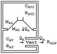
The 1-ported band pass box and the equivalent circuit diagram of its acoustic load.

The simplified transfer function of the 1-ported design behaves like a fourth-order band pass filter with slopes of 12 dB/octave at low frequencies and -12 dB/octave at high frequencies.

2-ported band pass box

The simulation of the 2-ported band pass box is similar to that of the 1-ported band pass box, but also has a vent in the second cavity. The second vent is connected in parallel with C_AV2 and R_AV2 and forms a symmetrical diagram, corresponding to the symmetrical design of the box. However, the two vents must be tuned to different frequencies. Just as the vent in the bass-reflex design provides the advantage of an extended low-frequency response compared to the closed box design, the second vent in the 2-ported design provides an extended low-frequency response as compared to the 1-ported box.

The radiation resistance is now calculated using the radius of the Vent1, so the highest helmholtz frequency should be assigned to Vent1, in this way this vent will dominate the radiation at higher frequencies.

The 2-ported band pass box and the equivalent circuit diagram of its acoustic load.

The simplified transfer function of the 2-ported design behaves like a sixth-order band pass filter with slopes of 24 dB/octave at low frequencies and -12 dB/octave at high frequencies.

Vent models

The tube vent can be modelled as a lumped mass or as a tube. The lumped mass model is accurate enough for low frequencies, and provides quick calculation of the response curves. The tube model provides extra information regarding resonances that occur in the tube, typically when tube the length corresponds to multiples of l/2. The vent can also be realised as a passive radiator.

Note that the co-oscillating air M_ALP is included in the model of the vent, but that the radiation resistance is treated separately in the other parts of the analogue circuit diagrams.

Symbol for the vent model used in Basta! It symbolises the vent mass and losses, and a compliance distributed along these. The vent can be modelled as a lumped mass, a tube or as a passive radiator.

Lumped model

The lumped model is activated by setting the number of sections of a vent to zero. In this case the vent is modelled by a mass M_AP and a resistance R_AP, the flow out of the tube is the same as the flow into the tube and thus the air in the tube is considered as being incompressible.

The equations for the acoustic mass and resistance of the port. Note that two end corrections first are removed from the mass, to model the air contained inside the tube. Thereafter the better model is added, this yields a better precision at higher frequencies.

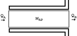
The lumped mass model and the equivalent circuit diagram of its acoustic properties.

In this case the air inside the vent is assumed to be incompressible and thus if air that flows into the vent at one end the same amount immediately flows out of the other end. This model is fast and accurate for low frequencies.

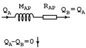
Tube model

If the air inside the tube is allowed be compressed, the model can simulate standing waves ("pipe resonances") within the tube. In its simplest form, the mass and resistance are split in two, and an acoustic compliance C_AP corresponding to the volume of air inside the tube is connected in between the two halves. This model can in principle simulate the first pipe resonance, but the resonance frequency will come out slightly too low.

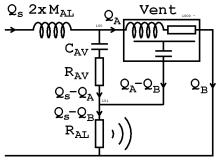
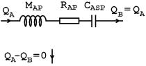
Setting the number of sections of the vent to one activates this simple tube model. The difference between incoming flow Q_A and outgoing flow Q_B represents the compression of the air inside the tube and flows out of the third branch.

The simple tube model of the vent and the equivalent circuit diagram of its acoustic properties.

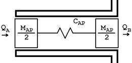
The tube model can be expanded to simulate higher order resonances as well. In this case the tube is split in several consecutive sections according to the figure. A higher number of tube sections will make the calculation process slower, but will increase the accuracy of the resonance frequencies.

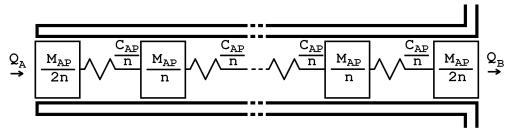
The generalised tube model of the vent and the equivalent circuit diagram of its acoustic properties.

Passive radiator

The vent can also be realised as a passive radiator. In this case, no tube resonances will appear. An extra compliance C_ASP is added, originating from the suspension of the cone. Just as for the lumped model the flow into the inside the radiator is the same as the flow out of the outside. Contrary to the lumped model of a tube, this model is accurate also for higher frequencies, as there are no tube resonances.

The passive radiator model of the vent and the equivalent circuit diagram of its acoustic properties.

Multiple loudspeaker elements

Basta! can simulate acoustic coupling of multiple loudspeaker elements, both in parallel and isobaric operation. By connecting n elements in parallel the maximum sound pressure of the system is increased a factor n², or 6 dB for two loudspeakers, 12 dB for four loudspeakers, etc. The efficiency is increased a factor n in the same configuration, but the box volume must be increased a factor n in order to maintain approximately the same frequency response as for the single loudspeaker system. As an alternative the loudspeakers may be mounted in the isobaric configuration. Using this configuration for two loudspeakers, the box volume can be halved, at the cost of a halved efficiency. However, since the electrical power handling capacity is doubled, and the maximum cone excursion remains the same, the maximum output sound pressure also remains the same.

In Basta! the electrical connection of the loudspeakers is expressed as the number of loudspeakers that are connected in series. They are always connected in such a way that each driver receives the same voltage. For example, if six drivers are used and three are connected in series, two such branches of three drivers are connected in parallel.

For multiple elements, the equivalent V_as, T, S_s, R_E and L_E values of the combined driver are derived from the single element. Given that

a is the number of elements that are connected in series, electrically,

b is 1 for parallel configuration 2 for isobaric configuration and

n is the total number of elements,

the new values are calculated as:

where sub-index "1" corresponds to the parameter of a single loudspeaker element.

b=1, n=2	b=2, n=2	b=2, n=4

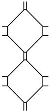
Acoustic connection of loudspeakers for some configurations. To the left, the loudspeakers are connected in parallel configuration, middle; isobaric configuration and to the right a combination of parallel and isobaric configuration.

a=2, b=1, n=2	a=2, b=2, n=2	a=1, b=1, n=2
a=1, b=2, n=2	a=3, b=1, n=6

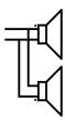
Electrical connection of some configurations. Note the reversed polarity for half of the elements in isobaric configuration.

Baffle step

When a driver is mounted on a baffle, the driver will roughly radiate in half space at high frequencies, but in full space at low frequencies. The result of this is an increase of 6 dB of the high frequencies. The response curve, starting at 0 dB at low frequencies and ending at + 6 dB at high frequencies, is commonly called the baffle step.

Basta! can model the baffle step, and uses a simplified version of the Geometric Theory of Diffraction (GTD). In short, a number of secondary sources are placed around the edge of the baffle, each having an amplitude and phase shift depending on the baffle shape. The resulting baffle step is thereafter added to the other response curves from Basta!.

Room gain

The room gain is represented by two poles and two zeroes and is added to the different response curves. The red explanatory curve below illustrates a pole pair at 20 Hz, Q=5 and a zero pair at 100 Hz, Q=5. Normally lower Q values are used; the default (black) curve has a smooth lift of the response towards lower frequencies.

Design suggestions

Basta! implements three commonly found design equations for vented boxes. These suggest the box volume and the vent tuning. The equations are:

Öhman:

Keele:

Margolis/Small:

For the closed box, the box volume that results in Butterworth response under free field conditions (ie Q=0.7071) can be suggested from

Maximum output level

Basta! allows for calculation of the maximum output level of the system. It is calculated based on these limits:

Maximum peak cone excursion

Maximum electric RMS power in R_E

Maximum RMS voltage from the power amplifier

Maximum RMS velocity in the vent(s)

Maximum RMS excursion of the vent(s)

The maximum output level is the highest level at which none of these limits are exceeded.

Curves

Curve	Unit	Note	Explanation
System response	dB	@ 1 m re 20 mPa	Sound pressure level as it would be measured straight in front of the loudspeaker
Max output level (MOL)	dB	@ 1 m re 20 mPa	Maximum possible SPL straight in front of the loudspeaker
Speaker voltage	V		The voltage across the speaker terminals
Speaker voltage at MOL	V		The voltage across the speaker terminals required to reach MOL
Amplifier voltage	V		The voltage across the amplifier terminals
Amplifier voltage at MOL	V		The voltage across the amplifier terminals required to reach MOL
Box (2) pressure	dB	re 20 mPa	The sound pressure inside the box. To measure this pressure with a microphone and compare it with the Basta! simulation can be a way to verify the response of a system, without having access to an anechoic chamber.
Box (2) pressure at MOL	dB	re 20 mPa	The sound pressure inside the box at max output level. This SPL is commonly very high, typically 140-160 dB.
Speaker response	dB	@ 1 m re 20 mPa	The part of the sound pressure level originating from the loudspeaker element.
Cone excursion	mm		The RMS movement of the loudspeaker cone
Cone velocity	m/s		The RMS velocity of the loudspeaker cone
Cone excursion at MOL	mm		The RMS movement of the loudspeaker cone at max output level
Cone velocity at MOL	m/s		The RMS velocity of the loudspeaker cone at max output level
Vent (2) response	dB	@ 1 m re 20 mPa	The part of the sound pressure level originating from the vent as it would be measured straight in front of the speaker.
Vent (2) excursion	mm		The RMS movement of the vent
Vent (2) velocity	m/s		The RMS velocity of the vent
Vent (2) excursion at MOL	mm		The RMS movement of the vent at max output level
Vent (2) velocity at MOL	m/s		The RMS velocity of the vent at max output level
Speaker baffle step	dB	94 dB added.	The baffle step that results from the dimensions of the baffle and the driver placement.
Vent (2) baffle step	dB	94 dB added.	The baffle step that results from the dimensions of the baffle and the vent placement. Usually this curve is of little practical concern, since the vent mostly radiates well below the frequencies where the baffle step is active.
Electrical impedance	W		This impedance is calculated as ua/ia, thus excluding the AC-bass circuit, but including the passive electric circuit.
Electrical inductance	mH		The reactive part of the electrical impedance, seen as an inductance ie divided by w. This curve can be useful if the manufacturer has specified the voice coil inductance as the inductance at two different frequencies.
Electrical resistance	W		The resistive part of the electrical impedance
Electrical reactance	W		The reactive part of the electrical impedance
RE power margin	dB		The level increase allowed to reach the power limit in RE.
Cone excursion margin	dB		The level increase allowed to reach the cone excursion limit.
Vent (2) excursion margin	dB		The level increase allowed to reach the vent excursion limit.
Vent (2) velocity limit	dB		The level increase allowed to reach the vent velocity limit.
Overall margin	dB		The level increase allowed without exceeding any of the limits. This curve is the difference between the MOL and system response curves.
Room gain	dB		The room gain (bass lift) approximation as selected on the room gain tab.

Note: If the baffle step is not enabled, all sound pressure levels outside the box are based on that the loudspeaker is mounted in a wall or floor and thus radiates in half space (2p). If the baffle step is enabled, the loudspeaker box is assumed to radiate in free field.

List of symbols

Symbol	Explanation
Rac	Resistance determining the resistive losses in the AC-bass system
Racneg	Negative output resistance of the AC-bass circuit
Lac	Inductance of the AC-bass circuit. Determines the effective compliance of the AC-bass system
Cac	Capacitance of the AC-bass circuit. Determines the effective mass of the AC-bass system
LL1,LL2	Inductors in passive lowpass filter
CL1,CL2	Capacitors in passive lowpass filter
RL1,RL2	Resistances in passive lowpass filter, eg in the inductors
LH1,LH2	Inductors in passive highpass filter
CH1,CH2	Capacitors in passive highpass filter
RH1,RH2	Resistances in passive highpass filter, eg in the inductors
Rs,Rp	Series and parallel resistances for passive attenuation
REC,CEC	Resistance and capacitance of the conjugate link
RE	DC resistance of the voice coil
LE	Inductance of the voice coil
n	Loss factor of the voice coil inductance
T	Force factor of the loudspeaker. Also known as Bl
RMS,CMS,MMS	Mechanical resistance, compliance and mass of the loudspeaker. MMS does not include any co-oscillating air.
Ss	Equivalent piston area of the loudspeaker cone
fs	Resonance frequency of the loudspeaker in free air
Vas	Equivalent volume of the loudspeaker. This volume would give a compliance equal to CMS, given the equivalent piston area Ss.
Qts	Total Q-value of the loudspeaker in free air, and zero series resistance.
rr	The radius of a circular membrane that corresponds to Ss.
ZE	The impedance of the voice coil, neglecting the effects of the mechanical system.
MALS, MALP, MALP2	The acoustic mass of the co-oscillating air for the loudspeaker, first vent and second vent. This mass corresponds to the reactive part of the radiation impedance.
RAL	The radiation resistance.